Correlation Analysis
Open from ‘3. Analysis Correlation Analysis‘.
The two-point spatial correlation function
measures the degree to which velocity fluctuations at two different locations are statistically related. When decays from 1 at to 0, the separation at which it crosses zero defines the integral length scale , a measure of the size of the largest energy-containing eddies (Pope, 2000). The temporal autocorrelation plays an analogous role in time, with the integral time scale .
Reference: Pope, S.B. (2000). Turbulent Flows. Cambridge University Press.
Selecting a reference
‘Point mode‘: left-click on the mean field to select a single reference point. Enable ‘ kernel average‘ to reduce sensitivity to noisy vectors at that point.
‘ROI mode‘: left-click and drag to draw a rectangle. The correlation is computed as a spatial average over the region.
Spatial correlation
In Point mode you see the full 2D correlation map and two independent 1D slice panels. In ROI mode only the 1D panels are shown. The computed and are displayed in the readout strip at the bottom of the window. A vertical dashed line marks the crossing lag used by the selected scale method; for the zero-crossing method, this line is placed at the lag where first crosses zero, while is reported as the integral of up to that crossing. Click ‘Show Diagnostic Plot‘ to see the cumulative integral of .
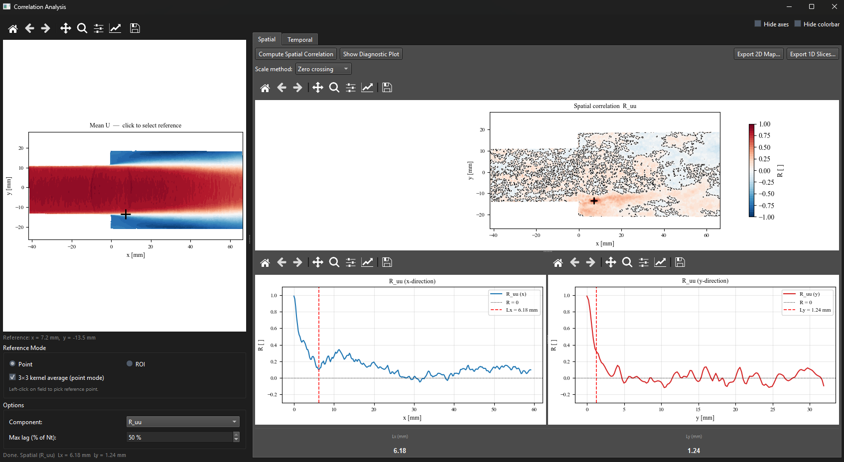
Figure 1:Correlation window in ROI mode showing in the - and -directions. The vertical dashed red line marks the zero-crossing lag used to compute the integral length scale. and are reported in the readout strip at the bottom.
Table 1:Integral scale methods.
| Method | When to use |
| Zero crossing | Clean, well-resolved correlations with a clear zero crossing. Standard choice. |
| Exponential fit | Noisy correlations without a clear zero crossing. Robust to noise in the tail. |
| 1/e point | Returns the lag at which first drops to (interpolated). |
| Domain integral | When no zero crossing exists and you want a conservative upper bound. |
Temporal correlation (TR only)
Results show vs time lag in milliseconds, with integral time scale and Taylor microscale marked.
Multi-case comparison
Spatial 1D slice and temporal correlation curves support CSV import and overlay (Chapter ??).