Vortex Identification
Open from ‘3. Analysis Vortex Identification‘.
Vortex identification methods seek to objectively define the boundary and core of a vortex from the instantaneous or mean velocity field. uPrime implements five scalar criteria, which can be broadly divided into gradient-based (Eulerian) methods and the integral-based Graftieaux criteria.
Gradient-based methods
All four gradient-based methods derive from the 2D velocity gradient tensor:
which is decomposed into its symmetric strain rate and antisymmetric rotation rate .
Vorticity : the simplest measure of local rotation, but nonzero in shear layers even without a vortex core.
Q-criterion (Hunt et al., 1988): . A vortex core is identified where , meaning rotation dominates strain. Q is the most widely used criterion in PIV literature.
Swirling strength (Zhou et al., 1999): the imaginary part of the complex eigenvalue of . Complex eigenvalues exist only where the flow is locally swirling; is therefore immune to pure shear contamination that inflates and in shear layers. uPrime multiplies by to retain rotation direction.
-criterion (Jeong & Hussain, 1995): identifies a vortex core as a connected region where the second eigenvalue of is negative. This criterion has a direct physical motivation: marks regions where the centrifugal tendency of the pressure field overcomes both strain and unsteady effects.
References: Hunt, J.C.R., Wray, A. & Moin, P. (1988). Eddies, stream, and convergence zones in turbulent flows. CTR Report CTR-S88, 193–208. Zhou, J., Adrian, R.J., Balachandar, S. & Kendall, T.M. (1999). Mechanisms for generating coherent packets of hairpin vortices in channel flow. Journal of Fluid Mechanics, 387, 353–396. Jeong, J. & Hussain, F. (1995). On the identification of a vortex. Journal of Fluid Mechanics, 285, 69–94.
Graftieaux functions
The functions (Graftieaux et al., 2001) are computed directly from the velocity vectors without differentiation, making them substantially more robust to PIV measurement noise:
where is a local neighborhood of points around , denotes the angle between two vectors, and is the local mean velocity over . Both functions are bounded between -1 and +1. The sign gives the rotation direction (+1 = CCW, -1 = CW). A vortex core is identified where –0.7; the vortex boundary is where . The neighborhood half-width (default 2, corresponding to a stencil) is user-adjustable.
Reference: Graftieaux, L., Michard, M. & Grosjean, N. (2001). Combining PIV, POD and vortex identification algorithms for the study of unsteady turbulent swirling flows. Measurement Science and Technology, 12(9), 1422–1429.
Field View tab
The threshold is expressed as a fraction of the field maximum, making it dataset-agnostic. The actual physical value is shown in the readout next to the slider. For the criteria the threshold has a universal meaning ( corresponds to the standard core boundary); for gradient-based criteria it is dataset-dependent and must be chosen by the user.
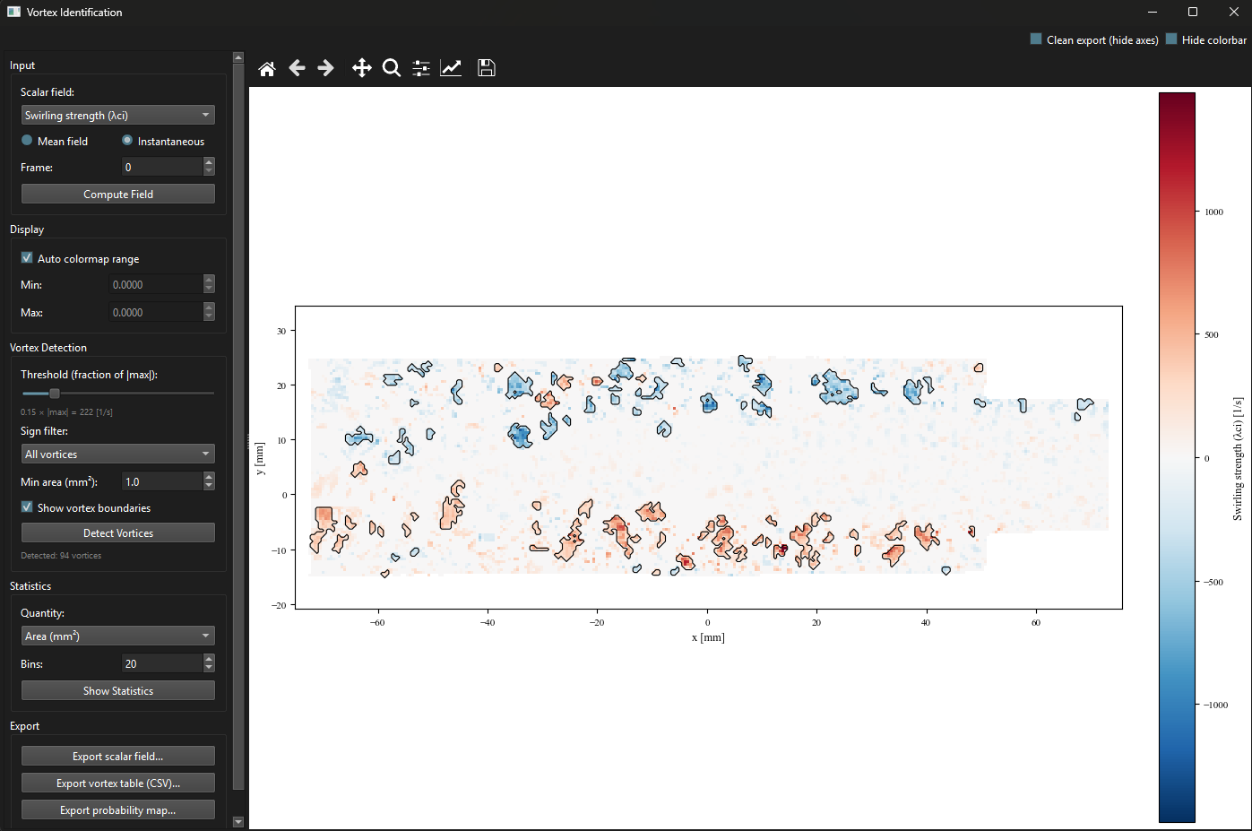
Figure 1:Vortex Identification window showing the swirling strength field for an instantaneous snapshot. Detected vortex boundaries (black contour lines) are overlaid on the colormap. The threshold is set to 15% of the field maximum. Red regions indicate positive (CCW) rotation; blue regions indicate negative (CW) rotation. A total of 94 vortices are detected above the minimum area threshold.
Vortex Statistics tab
After clicking ‘Show Statistics‘, two plots appear: a spatial probability map showing how often a vortex is detected at each grid point across all snapshots, and a histogram of the selected per-vortex quantity (area, circulation, or aspect ratio) with positive and negative vortices shown separately in red and blue.
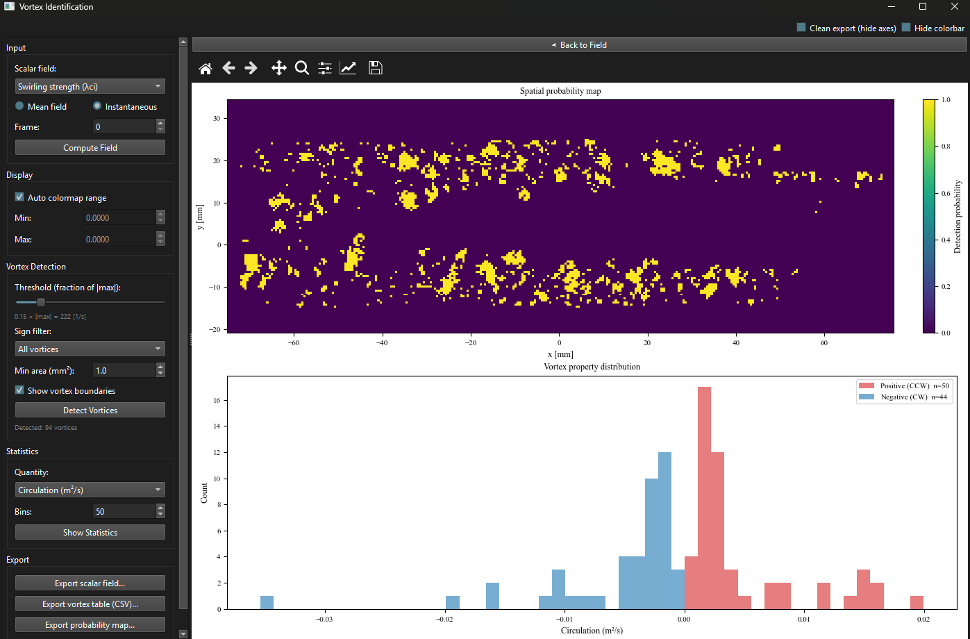
Figure 2:Vortex Statistics view. Top: spatial probability map showing the fraction of snapshots in which a vortex is detected at each grid point (viridis colormap, 0–1). Yellow regions indicate persistent vortex locations concentrated in the shear layers. Bottom: circulation histogram for 94 detected vortices (50 CCW in red, 44 CW in blue). The near-symmetric distribution about zero is consistent with a turbulent shear layer with no mean rotation bias.
Exporting
Click ‘Export scalar field…‘ to save the scalar field as a Tecplot .dat file. Click ‘Export vortex table (CSV)…‘ to save a per-vortex table with columns: vortex ID, centroid position, area, sign, circulation, aspect ratio, and frame index. The default filename now reflects the active criterion (e.g. vortex_lambda_ci_dataset.csv). This CSV is designed to be imported into post-processing scripts for vortex tracking or further statistical analysis.