Getting Started
What is uPrime?
uPrime reads Tecplot .dat files exported from LaVision DaVis, and MATLAB .mat files containing PIV or CFD velocity fields. It provides a graphical interface for turbulence post-processing. You do not need to know Python, MATLAB, or any programming language to use it. Everything is point-and-click.
The workflow is always the same:
Load your snapshots (
.dator.mat).Set the acquisition type and sampling frequency.
Align the coordinate system if needed.
Verify statistical convergence in the ‘Mean & Convergence‘ module.
Open any analysis module and explore your data.
What uPrime can do
Load 2D2C and 2D3C (stereo) PIV data from multiple
.datfiles or a single.matfile.Display mean velocity fields, standard deviation, vorticity, velocity vectors, and streamlines.
Plot mean velocity line profiles (free, horizontal, vertical) and verify cumulative-statistics convergence at any picked point.
Compute all Reynolds stress components with 2D maps, line profiles, and uncertainty bands.
Compute and plot the full TKE budget (production, convection, turbulent diffusion, residual) with selectable term visibility.
Perform spatial, temporal, and space-time spectral analysis.
Compute two-point spatial and temporal correlations with integral length and time scales.
Analyze turbulence anisotropy via the Lumley triangle and barycentric maps (stereo only).
Perform Proper Orthogonal Decomposition (POD) with energy spectra, mode shapes, and flow reconstruction.
Perform Dynamic Mode Decomposition (DMD) with frequency spectra and spatial mode visualization (TR only).
Identify vortex cores and boundaries using five scalar criteria: vorticity, Q-criterion, swirling strength, , and / (Graftieaux).
Compute probability density functions of the velocity components and their fluctuations at a point, along a line, in a region of interest, or over the whole field, with skewness and flatness.
Map forward-flow and reverse-flow probability (backflow coefficient) to locate and quantify intermittent separation.
Plot binary space-time maps of the fluctuation sign along a line to visualise the passage of coherent structures (TR only).
Decompose the Reynolds shear stress into ejections, sweeps, and interactions by quadrant analysis, with a hole-size sweep and joint PDF.
Import multiple cases (CSV) and overlay them in Reynolds stress, TKE budget, spectra, correlation, anisotropy, and mean velocity plots for direct visual comparison.
Apply and manage non-destructive spatial masks.
Correct camera calibration misalignment, shift the coordinate origin, and mirror the dataset.
Export all results as Tecplot
.dator.csvfiles, and figures as PNG (300 DPI), PDF, or SVG with editable text.
System requirements
Minimum system requirements.
| Item | Requirement |
| Operating system | Windows 10/11 (primary); macOS 12+; Linux (Ubuntu 20+) |
| Python | 3.10 or later (source installation only) |
| RAM | 8 GB minimum; 16 GB or more recommended for large datasets |
| Display | 19201080 or larger strongly recommended |
| Python dependencies (source installation) | |
numpy | Array operations and numerical core |
scipy | Signal processing and spectral analysis |
matplotlib | Plotting and figure export |
PyQt6 | Graphical user interface |
pyfftw | Fast Fourier transforms (accelerates spectral analysis) |
h5py | Read v7.3 (HDF5-based) .mat files |
Installation
Option A: Windows executable (recommended for non-developers)
Download uPrime_v0.7.1.exe from the GitHub Releases page and double-click to launch. No Python or any other software is required.
Option B: Run from source
Clone the repository:
git clone https://github.com/CmdrRyder/uPrime.git
cd uPrime
Install dependencies:
pip install -r requirements.txtLaunch:
python main.py
Input file formats
uPrime accepts two file formats: Tecplot ASCII .dat (one snapshot per file) and MATLAB .mat (full time series in a single file). The file type is auto-detected from the extension.
Tecplot ASCII (.dat)
uPrime reads Tecplot ASCII .dat files in the standard DaVis export format. Each file contains one PIV snapshot. Select multiple files at once to load a full time series.
uPrime automatically reads the physical units from the variable name strings in the file header (e.g. "x [mm]", "Velocity u [m/s]"). If units are not specified in the header, it defaults to millimetres for coordinates and m/s for velocity. All internal computations are performed in SI units regardless of the input.
MATLAB (.mat)
uPrime also loads MATLAB .mat files. Both classic v5/v7 (read via scipy.io) and v7.3 (HDF5-based, read via h5py) are supported. Format detection is automatic.
One
.matfile contains the entire dataset (all snapshots).Velocity arrays must have shape
(Ny, Nx, N_snap). The loader detects and corrects the alternative(Nx, Ny, N_snap)ndgrid convention automatically.Coordinate arrays
xandycan be 1D vectors or 2D meshgrid arrays. Transposed meshgrids are auto-corrected; orientation is determined primarily from the variance pattern in the data, with shape comparison as a fallback.Variable names are auto-detected. The recognized candidates (case-insensitive) are:
x, X, xc, xxfor ;y, Y, yc, yyfor ;u, U, Vx, vxfor ;v, V, Vy, vyfor ;w, W, Vz, vzfor (optional);isValid, isvalid, mask, valid, IsValidfor the validity mask (optional). Extra variables are ignored.Multiple snapshots required. Single-snapshot files (where the velocity array is 2D, or has
N_snap= 1) are detected from metadata and rejected with a clear error before any data is loaded.
When you select a .mat file, uPrime reads only the variable names and shapes (no data) and shows the variable confirmation dialog (Figure 1). The dialog appears within seconds even for very large files.
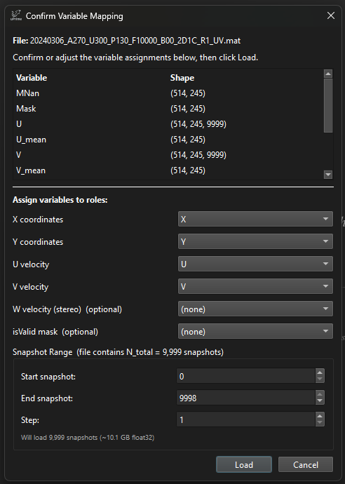
Figure 1:.mat variable confirmation dialog. The top panel lists every variable in the file with its shape. Six dropdowns map the file variables to uPrime’s expected roles (, , , , , isValid); auto-detected matches are pre-filled. The bottom panel sets the snapshot subset to load (start, end, step), with a live readout of the resulting count and estimated memory size. Click ‘Load‘ to confirm and start the actual data read.
Snapshot subset.
The dialog includes Start, End, and Step spinboxes. They allow loading only a slice (e.g. snapshots 0–999) or a strided subsample (e.g. every 10th snapshot from 0 to 9999). The estimated in-memory size updates live. This is useful for preliminary inspection of very large files before committing to the full load.
Mask convention.
A ‘Mask convention‘ dropdown sits next to the isValid selector. The default, ‘1 = valid (uPrime default)‘, matches the .dat convention. If your file uses the opposite convention (for example a Mask variable where 1 marks points to exclude), select ‘1 = invalid (mask out)‘. uPrime applies the chosen convention directly, with no auto-detection. After loading, the status bar warns if the resulting masked fraction is extreme (below 5% or above 95%); if that warning is unexpected, reload with the other convention.
Progress feedback.
For v7.3 files (HDF5), the read is chunked snapshot-by-snapshot and the progress bar advances determinately. For classic .mat files, the read is a single blocking call from scipy.io, so a busy indicator is shown along with the file size in the status bar. After the read, the status bar prints a confirmation listing the chosen variables and snapshot count, for example:
Loaded .mat: x=X, y=Y, u=U, v=V, w=(none), isValid=(none), N=1000 of 9999 (range 0:9990 step 10)
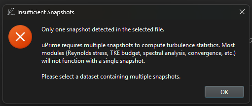
Figure 2:Error dialog shown when a .mat file contains only one snapshot. The check is performed on the metadata before any data is loaded, so the error appears immediately regardless of the file size.