Main Window
Overview
When uPrime launches you will see a welcome screen. The sidebar on the left is your control panel. All steps are numbered in the order you should use them.
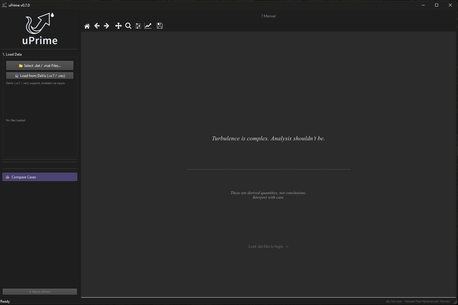
Figure 1:uPrime v0.7.0 welcome screen on launch. The sidebar shows Step 1 (Load Data) only. The ‘? Manual‘ button is visible in the top right. Load .dat or .mat files from the sidebar to begin.
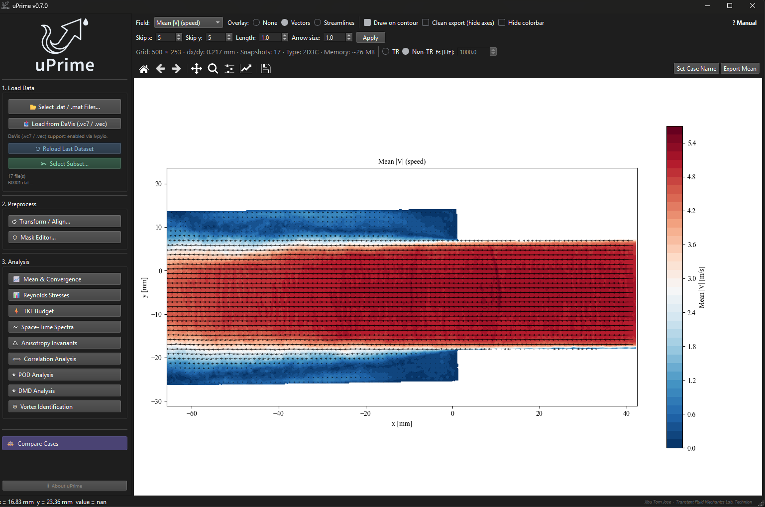
Figure 2:Main window after loading a dataset. The Analysis panel lists modules in the recommended order of use, beginning with ‘Mean & Convergence‘ for verifying statistical convergence before moving to higher-order statistics.
Step 1: Load Data
Click ‘Select .dat / .mat Files…‘ to open a file browser. You can select multiple .dat files (one snapshot each) or a single .mat file (full time series). The file type is auto-detected from the extension.
For .dat loads, a subsampling dialog appears next (see Section ??). For .mat loads, the variable confirmation dialog appears (see Section ??).
After loading, the acquisition-type dialog appears. Set ‘TR‘ (time-resolved) or ‘Non-TR‘ and enter the sampling frequency if TR.
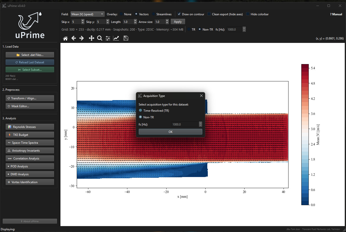
Figure 3:Acquisition type dialog shown automatically after each data load. Select TR and enter to enable temporal analysis modules. The spinbox is greyed out when Non-TR is selected.
Step 2: Preprocess
Click ‘Transform / Align…‘ to open the coordinate correction tool. This is where you fix camera tilt, shift the coordinate origin, and optionally mirror the dataset. Always do this before running any analysis. Full details are in Chapter ??.
Click ‘Mask Editor…‘ to draw additional spatial masks over regions you want to exclude from analysis (e.g. reflections, shadows, or wall regions not detected by the DaVis isValid flag). Masks are non-destructive: the raw velocity data is never modified. Toggling a mask on or off does not require reloading.
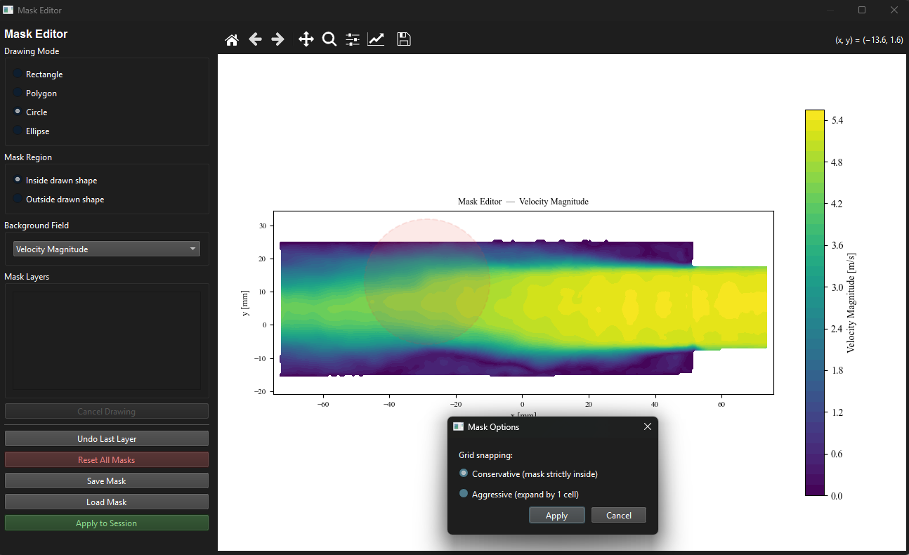
Figure 4:Mask Editor window. The user is drawing a polygon (red) over a region to exclude. Drawing modes include Rectangle, Polygon, Circle, and Ellipse. The mask can be applied inside or outside the drawn shape. Multiple layers can be stacked and each can be undone independently.
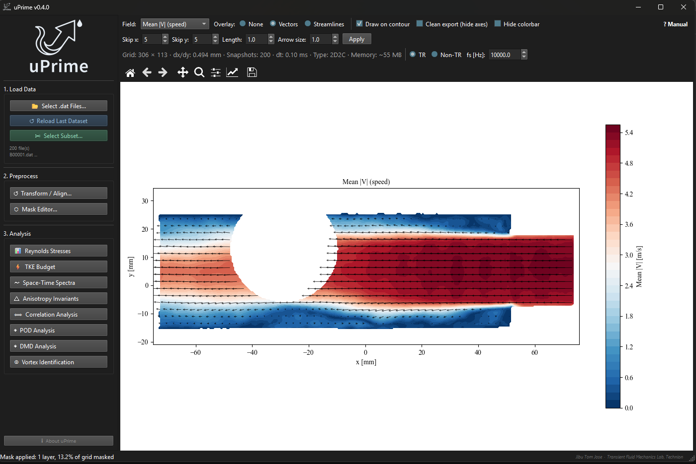
Figure 5:Main window after applying a drawn mask. The masked region is shown in white. The status bar at the bottom reports the number of mask layers and the fraction of the grid that is masked.
Step 3: Analysis
Click any analysis button to open that module in its own window. Multiple analysis windows can be open at the same time and can be compared side by side. The recommended starting point is ‘Mean & Convergence‘ (Chapter ??); from there proceed to Reynolds stresses, TKE budget, and the higher-order modules as appropriate.
All heavy computations (POD, DMD, TKE budget, correlation, vortex identification, probability analysis) run in a background thread so the main window remains fully responsive during computation. A progress indicator appears below the compute button while the calculation is in progress.
Acquisition type and sampling frequency
The acquisition type and sampling frequency are set in the dataset info ribbon at the top of the main window, immediately below the field options strip. A dialog to set these values also appears automatically after each data load.
‘TR‘: snapshots are acquired at a fixed rate. Enter in Hz (enabled only for TR). Temporal analyzes (temporal spectra, temporal correlation, POD temporal coefficients, DMD) become available.
‘Non-TR‘: snapshots are statistically independent (e.g. double-frame PIV). Temporal analyzes are greyed out.
Dataset info ribbon
A compact info strip appears just below the options strip after loading:
Grid: 507 248 dx/dy: 0.165 mm Snapshots: 2000 dt: 0.10 ms Type: 2D2C Memory: ~2012 MB
Grid: number of velocity vectors in and .
dx / dy: spatial resolution in mm. For
.matfiles this is estimated from the coordinate arrays using the median of differences (robust to small rounding at the edges). A non-uniform grid (more than 1% variation in spacing) triggers a status-bar warning, since FFT and Welch spectra assume uniform grids.Snapshots: how many snapshots are currently active (reflects subsampling).
dt: time between frames in milliseconds (TR data only; updates if or stride changes).
Type:
2D2Cfor planar PIV;2D3Cfor stereo PIV with .Memory: estimated RAM used by the velocity arrays. For datasets exceeding 4 GB, this reflects the size of the memory-mapped file on disk rather than physical RAM consumed (see Section ??).
Field viewer
The right panel shows the selected velocity field as a filled contour plot with optional velocity vectors.
Display controls
Field viewer display controls.
| Control | Description |
| Field | Quantity to show: Mean U/V/W, speed , vorticity, Std(U), Std(V) |
| Overlay | None, Vectors, or Streamlines |
| Draw on contour | When checked, overlays the selected overlay on the filled contour |
| Clean export | Hides all axis labels, tick marks, and the plot title for a clean exported image |
| Hide colorbar | Removes the colorbar from the plot |
| ? Manual | Opens the user manual PDF |
Streamlines
Streamlines trace the instantaneous mean velocity field and give a cleaner visual impression of the flow topology than arrow vectors, especially in regions with complex recirculation.
Toolbar
Toolbar button functions.
| Button | Function |
| Home | Resets the view to the original limits, regardless of zoom history |
| Back / Forward | Step through zoom history |
| Pan | Click and drag to pan the view |
| Zoom | Click and drag a rectangle to zoom in |
| Save | Save the figure as PNG (300 DPI), PDF, or SVG |
Saving figures
Click the Save button in the toolbar. PNG is saved at 300 DPI. PDF and SVG use vector graphics; all text is saved as editable text and can be restyled in Adobe Illustrator or Inkscape.
Export menu
The ‘Export‘ menu in the menu bar provides one-click export of the time-averaged mean field as a Tecplot ASCII .dat file. The exported file contains , , , and (for stereo data) on the original grid, ready for use in CFD validation, plotting in Tecplot, or import into other PIV tools.
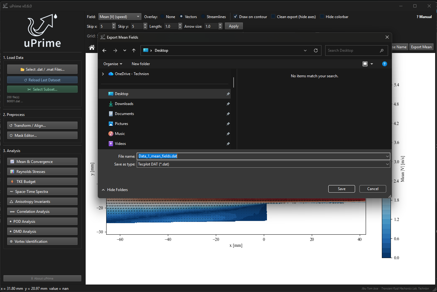
Figure 6:Main window ‘Export‘ menu showing the Tecplot ASCII mean field export option.
Snapshot subsampling and large dataset handling
A subsampling dialog appears whenever .dat files are selected, giving you control over how many snapshots to load. The same controls (start, end, step) are available inside the .mat variable confirmation dialog (Section ??).
Load all: load every file in the selection.
Stride: load every -th snapshot. Stride 5 on a 10,000-snapshot dataset gives 2000 samples, which is sufficient for mean fields, Reynolds stresses, and correlations.
Limit: load only the first snapshots.
The dialog shows the estimated snapshot count and memory usage, updating live as you change the options.
After loading, click ‘Select Subset…‘ to adjust the active snapshot range without re-reading from disk.
Large dataset handling (datasets exceeding 4 GB)
When the estimated dataset size after subsampling exceeds 4 GB, uPrime automatically switches to a memory-mapped loading strategy. Instead of loading all velocity data into RAM, uPrime writes the data to a temporary binary file on your system’s temp drive (typically C:\ Users\ username\ AppData\ Local\ Temp) and accesses it as needed. The actual path is shown in the warning label inside the subsampling dialog.
The key practical differences when memory-mapped loading is active:
Initial load is slower: uPrime writes the full dataset to disk before opening it. On a fast SSD, expect 30–90 seconds for a 10 GB dataset in addition to the normal file reading time.
All analysis works normally: POD, DMD, TKE budget, spectra, correlation, and vortex identification all function identically. Memory-mapped arrays behave like regular numpy arrays.
RAM usage is reduced: only the pages of data currently being accessed are held in RAM. The operating system manages this automatically.
Do not load from external drives: if your
.datfiles are on an external HDD, copy them to a local drive first. Reading from an external drive while also writing the memory-mapped cache to the temp drive simultaneously will be very slow.