Reynolds Stress Analysis
Open from ‘3. Analysis Reynolds Stresses‘.
In turbulent flows, the instantaneous velocity can be decomposed into a time-averaged mean and a fluctuating component , such that . The Reynolds stress tensor quantifies the statistical intensity and directionality of these fluctuations and appears as a closure term in the Reynolds-Averaged Navier-Stokes (RANS) equations (Pope, 2000):
The diagonal components , , are the normal stresses, directly related to the turbulent kinetic energy by . The off-diagonal components , , are the shear stresses, which are responsible for the turbulent momentum transfer across shear layers and boundary layers.
For 2D2C data, only , , and are available. All six components are computed for stereo (2D3C) data.
Reference: Pope, S.B. (2000). Turbulent Flows. Cambridge University Press.
2D contour map
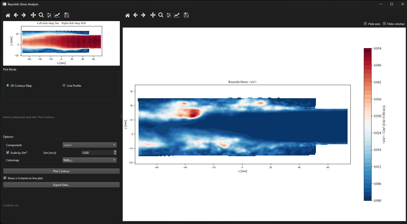
Figure 1:Reynolds stress window in 2D contour mode showing . The mean field is shown in the small reference panel on the left.
Line profile
All available stress components are plotted together. Check ‘Show band‘ to display uncertainty bands. From v0.5.0 onward this checkbox is unchecked by default; the bands tend to crowd plots when multiple cases are overlaid for comparison.
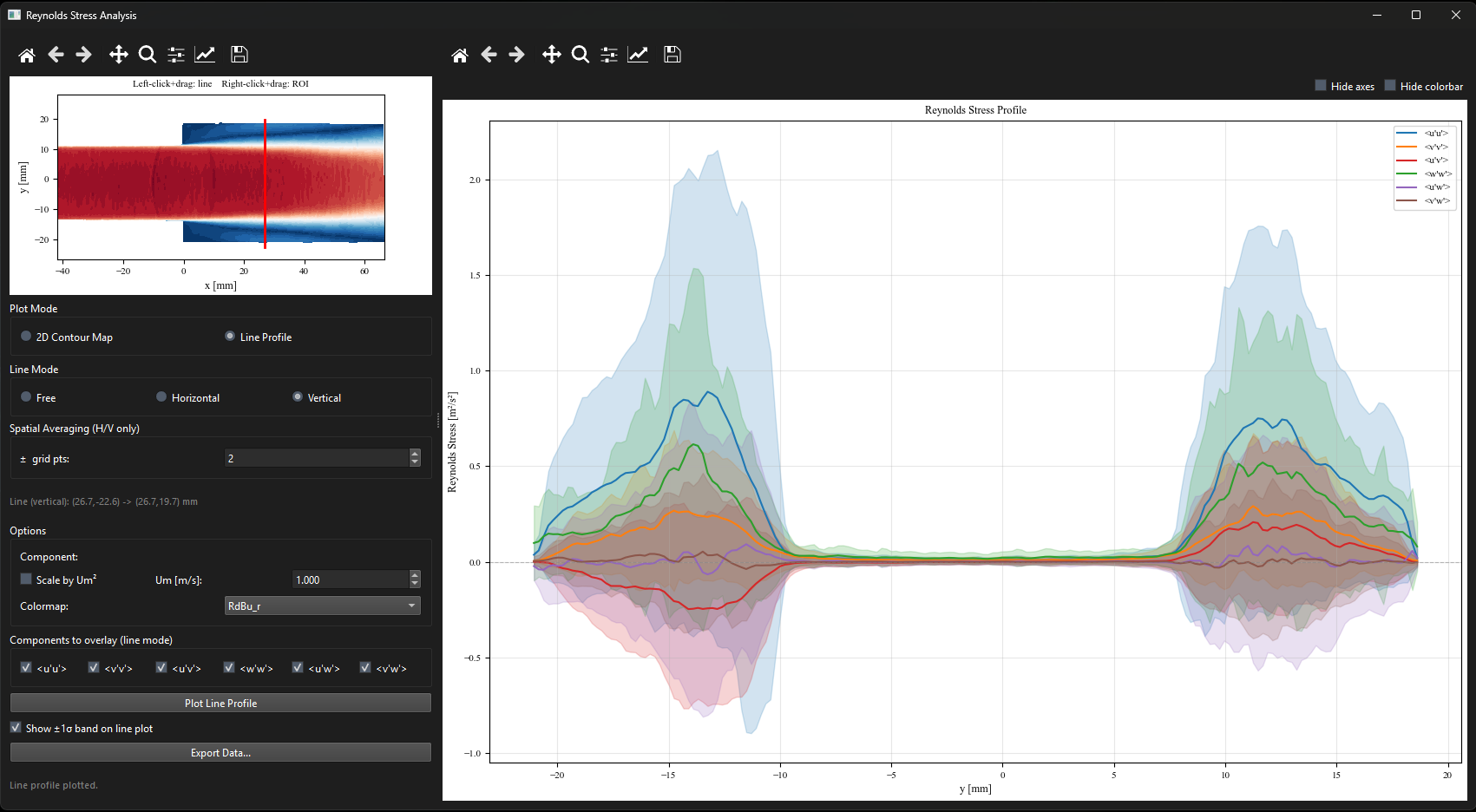
Figure 2:Reynolds stress window in line profile mode. All stress components are plotted simultaneously in different colors. Optional shaded bands show statistical uncertainty (toggle in the side panel).
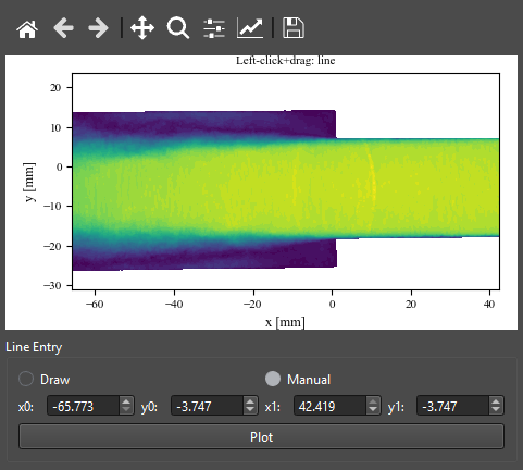
Figure 3:Manual line-coordinate entry (v0.7.0). In any Line Profile mode the endpoints can be set numerically as and instead of, or in addition to, click-and-drag. The same coordinate boxes appear in Reynolds Stress, TKE Budget, and Mean Velocity line profiles, so an identical line can be reproduced exactly across datasets.
Multi-case comparison
The Reynolds Stress window supports importing CSV exports from previous sessions and overlaying them on the current plot. See Chapter ?? for the full workflow. The same Import Case, Edit Styles, Manage Cases, and Export All Cases controls apply.
Exporting
Click ‘Export Data…‘ to save all stress components simultaneously in a single Tecplot .dat file or as a CSV.